Taylor Dispersion Analysis (TDA) is a microcapillary flow-based technique whereby a nanoliter-scale sample pulse is injected into the laminar flow of run buffer, which then spreads out axially due to the combined actions of convection and radial diffusion. Detection of the equilibrium concentration profile (or Taylorgram) of the dispersed sample pulse allows the molecular diffusion coefficient and hence hydrodynamic radius of solute molecules to be calculated. An instrument implementation utilising a UV area array detector in combination with two detection windows enables selective, mass-weighted sizing of small molecules, peptides and proteins, and samples with mixtures of these species. The TDA technique further lends itself to novel (label-free) analysis of the interactions, conformation and stability of proteins and other target molecules within complex biologically-relevant media e.g. excipient and/or surfactant-laden bioformulations, and aggregated solutions.
1. Introduction
Taylor Dispersion Analysis (TDA) is a fast and absolute method for determining the diffusion coefficients (and hence the hydrodynamic radii) of molecules. The method, sometimes referred to as Taylor-Aris dispersion, was first described by Taylor in his classic paper1, where he measured the dispersion of a pulse of solute injected into a flowing fluid in a capillary. In 1956, Aris developed the method further by accounting for the longitudinal diffusion of the molecules2. Taylor’s deduction was based on his observation that the dispersion of the solute occurs via a combination of the radial diffusion of the molecules and convection due to the cross-sectional velocity of the fluid. A pressure-driven fluid in a cylindrical tube flows under Poiseuille laminar conditions3. This implies that the velocity of the fluid decreases radially from a maximum umax at the centre of the cylinder to a minimum umin at the walls of the cylinder. The effect of this velocity distribution on the profile of an injected solute pulse is illustrated in Figure 1.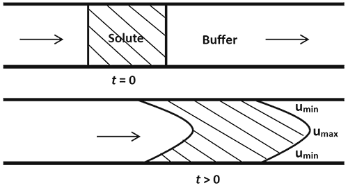
Figure 1: Axial spreading of the solute due to convection The axial spreading of the solute pulse along the direction of flow (indicated by the arrows) is illustrated in Figure 1. This is known as convection. The front and back ends of the pulse which start out as sharp interfaces become parabolic in shape due to the laminar flow of the fluid. In the absence of any other dispersion mechanism, the axial spreading will continue in time and the solute molecules will be increasingly dispersed over the length of the tube i.e. the injected solute pulse would develop an asymmetric concentration distribution. Diffusion is the movement of solute molecules from regions of higher concentration to regions of lower concentration. Hence, it is often thought of as a spreading mechanism. Counterintuitively, however, the role of radial diffusion (i.e. diffusion perpendicular to the fluid flow) in Taylor Dispersion is to limit the axial spreading due to convection. Figure 2 illustrates why this is the case.
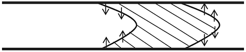
Figure 2: The role of radial diffusion
The directions of the radial diffusion of the solute molecules are highlighted in Figure 2. At the front end of the pulse, the solute concentration is higher at the centre of the cylinder than at the cylinder walls. Hence, the solute molecules diffuse radially toward the cylinder walls. Since the solute molecules at the centre are travelling much faster than the molecules at the walls, the average axial velocities of these molecules are reduced by the diffusion. At the rear end of the pulse, the solute concentration is higher at the walls than at the centre, so the molecules diffuse radially toward the centre. This results in an increase in the average axial velocities of the diffusing solute molecules. Overall, the effect of radial diffusion is to slow the leading interface and accelerate the trailing interface thereby keeping the solute distribution more compact in the axial direction than it would have been under convection alone. The axial spreading due to the combination of both radial diffusion and convection ultimately results in the injected solute pulse developing a symmetrical concentration distribution, and is known as Taylor Dispersion.
From the preceding discussion, it can be deduced that solutes with small diffusion coefficients will be dispersed more than those with larger diffusion coefficients and vice versa. This is because whilst the diffusion coefficient (and hence the amount of diffusion) varies with the type of molecule, the amount of convection experienced is the same for all molecule types.
It should be noted that the solute molecules also diffuse in a direction parallel to the flow. Typically, this contribution is small in comparison to the overall axial dispersion. However, it was quantified by Aris in 1956 and in cases where it is accounted for, the mechanism is known as Taylor-Aris dispersion2.
2. Taylor Dispersion Analysis
As described above, the amount of dispersion of a solute in a stream of solvent is inversely related to its diffusion coefficient. The amount of dispersion is a function of both the time elapsed as well as the position of the solute within the flow. This relationship is described by Equation 1 which relates the variation of the solute concentration C in time t to its variation with its axial position x along the capillary. Note that C is the solute concentration averaged across the capillary diameter in the direction y, perpendicular to the flow axis x as illustrated in Figure 3.
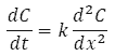
Equation 1
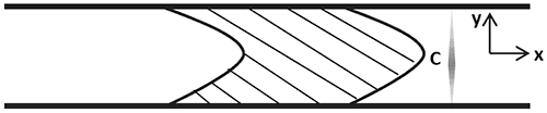
Figure 3: The concentration is averaged over the y-direction, perpendicular to the flow axis X
The constant k is known as the dispersion coefficient and is related to the diffusion coefficient D by:

Equation 2
where r is the capillary radius and u is the mean speed of the fluid flow.
Note the inverse relationship between the dispersion and diffusion coefficient as predicted qualitatively in Section 1. The hydrodynamic radius Rh is inversely related to the diffusion coefficient via Stokes’ law and is given by:

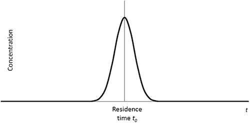
Equation 3 where kB is Boltzmann’s constant, T is the temperature and h is the viscosity of the solvent. There are a range of possible solutions to Equation 1 which depend on the initial conditions. The solutions describe the evolution of the concentration profile as a function of time and space during the dispersion. An example of such a solution is illustrated in Figure 4.
>> Free download of the full Application Note as PDF
Malvern Instruments provides the materials and biophysical characterization technology and expertise that enable scientists and engineers to understand and control the properties of dispersed systems. These systems range from proteins and polymers in solution, particle and nanoparticle suspensions and emulsions, through to sprays and aerosols, industrial bulk powders and high concentration slurries. Used at all stages of research, development and manufacturing, Malvern’s materials characterization instruments provide critical information that helps accelerate research and product development, enhance and maintain product quality and optimize process efficiency. Our products reflect Malvern’s drive to exploit the latest technological innovations and our commitment to maximizing the potential of established techniques. They are used by both industry and academia, in sectors ranging from pharmaceuticals and biopharmaceuticals to bulk chemicals, cement, plastics and polymers, energy and the environment. Malvern systems are used to measure particle size, particle shape, zeta potential, protein charge, molecular weight, mass, size and conformation, rheological properties and for chemical identification, advancing the understanding of dispersed systems across many different industries and applications. Headquartered in Malvern, UK, Malvern Instruments has subsidiary organizations in all major European markets, North America, Mexico, China, Japan and Korea, a joint venture in India, a global distributor network and applications laboratories around the world. www.malvern.com severine.michel@malvern.com
Newsletters
Receive the latest pharmaceutical news, personalities, education, and career development – weekly to your inbox.